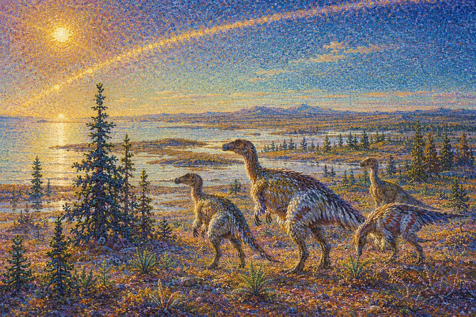
The Tilted Earth That Warmed the Dinosaur Arctic

A Japanese team has reproduced the warmth recorded by Late Cretaceous fossils by allowing Earth’s orbit to vary across its natural range. The result does not replace carbon dioxide. It shows how axial tilt, an ice-free world and a vanished continental map worked together to make northern high latitudes unusually responsive to sunlight.

Imagine winter on the Arctic coast about 70 million years ago. The sun still disappears. Darkness still stretches across weeks and months; no rearrangement of continents can repeal astronomy. Yet this is not the white desert familiar from satellite photographs. Rivers move through floodplains. Conifers and broad-leaved plants form forests. Hadrosaurs, horned dinosaurs and small feathered hunters leave bones, tracks and nesting evidence at latitudes where modern landscapes are locked in permafrost.

For generations, that world has posed an uncomfortable test. Rocks and fossils insist that the polar climate of the Late Cretaceous was much warmer than today. Many numerical models, when given plausible greenhouse-gas concentrations, have produced an Arctic too cold or an equator-to-pole temperature difference too steep. Either the geological thermometers were being misread, the models were missing an amplifier, or the experiments had frozen a moving part of the ancient Earth.

A study published online July 22 in Geophysical Research Letters identifies one such moving part. Taro Higuchi of the Earth-Life Science Institute at Science Tokyo, Ayako Abe-Ouchi and Wing-Le Chan of the University of Tokyo’s Atmosphere and Ocean Research Institute, and Ryouta O’ishi of Science Tokyo used the Japanese coupled climate model MIROC4mV to simulate the Maastrichtian, the final age of the Cretaceous. Instead of assigning the ancient planet today’s orbital geometry, they explored the natural range of orbital configurations.

When they did, the model could reproduce proxy-based estimates of polar surface temperature. More revealingly, the same orbital changes produced a much larger temperature response under Maastrichtian geography than under the modern continental map. The strongest contrast involved obliquity—Earth’s axial tilt. In the broad northern lands of the Late Cretaceous, without Greenland- or Antarctic-scale ice sheets, an increase in tilt warmed northern high latitudes several times more strongly than in the modern-geography comparison.

Carbon dioxide set the warm stage. Orbit changed where and when sunlight arrived. Cretaceous geography determined how forcefully the Arctic answered.

The experiment that made the ancient Earth move again

The paper, “Enhanced Orbital-Forcing Sensitivity of Northern High Latitude Temperatures in the Late Cretaceous Relative to Modern Geography,” is built around a controlled comparison. MIROC4mV couples atmosphere, ocean, sea ice, land and dynamic vegetation. The researchers supplied it with a reconstruction of Maastrichtian land, seafloor and coastlines, appropriate carbon dioxide and solar conditions, and combinations of the three principal orbital elements: eccentricity, precession and obliquity.

They then performed corresponding experiments with modern geography. That second Earth is essential. If the orbital response grew simply because the model was warm, the result would say little about continents. By comparing climates under the same carbon dioxide and solar conditions but different geography, the team could ask a sharper counterfactual: how would the same celestial nudge act on two different planetary surfaces?

The answer was not uniform. The Maastrichtian northern high latitudes were especially sensitive. A large fraction of the region was land rather than ocean, and the planet lacked the massive continental ice sheets that dominate today’s polar albedo and elevation. Land has less effective heat storage than the ocean and responds strongly to seasonal solar input. The reconstructed surface therefore converted a tilt-driven change in summer sunlight into a larger regional temperature swing.

~70 million yearsThe Maastrichtian world simulated in the new study.

22.1°–24.5°Earth’s approximate obliquity range over the last million years.

~41,000 yearsThe characteristic rhythm of the axial-tilt cycle.

Several timesThe reported amplification of high-latitude warming under Cretaceous versus modern geography.

Three slow dials around the Sun

“Earth’s orbit” is not one dial. Eccentricity describes how circular or elliptical the path around the Sun is. Precession changes the direction in which the spinning axis points and, together with the rotation of the orbital ellipse, shifts the seasons relative to perihelion and aphelion. Obliquity is the angle between Earth’s rotational axis and the perpendicular to its orbital plane—the tilt that creates the seasons.

Over the last million years, obliquity has varied between roughly 22.1 and 24.5 degrees on a cycle of about 41,000 years. Greater tilt gives high latitudes more summer sunlight and less winter sunlight. It strengthens seasonality; it does not turn off polar night. Nor does it add a large new annual total of solar energy to the whole planet. It redistributes energy by latitude and season, after which snow, ice, vegetation, clouds, atmosphere and ocean decide what becomes of the perturbation.

That distinction is the heart of orbital climate science. A modest astronomical rhythm can pace major environmental change when feedbacks and boundary conditions are ready to amplify it. The new work extends that logic far beyond the Quaternary ice ages. Its Cretaceous Arctic is not merely warmer under one favorable orbit; its geography makes the entire high-latitude system more sensitive across the range of possible orbits.

Element	What changes	Why the high latitudes care
Obliquity	Axial tilt, with a characteristic cycle near 41,000 years.	Higher tilt sends more summer radiation toward the poles and increases seasonal contrast.
Precession	The season in which a hemisphere points toward the Sun near perihelion.	It intensifies summer in one hemisphere while moderating it in the other.
Eccentricity	The orbit’s shape, from nearly circular to more elliptical.	It modulates the strength of precession and the Earth–Sun distance contrast.
Paleogeography	The location, elevation and area of land, oceans and gateways.	It controls heat storage, currents, snow and sea ice, turning the same orbit into a different climate.

A planet whose map has been erased

The Maastrichtian ran from about 72.2 to 66 million years ago. The Atlantic was opening, India was moving northward as an island continent, and high seas flooded broad continental interiors. North America was divided for much of the Late Cretaceous by the Western Interior Seaway. The coastlines and ocean gateways that route modern heat did not exist in their present form.

The northern polar region also contained a larger area of land than today’s ocean-centered Arctic. That fact changes the annual energy ledger. Ocean mixes solar heat downward and releases it slowly; land warms and cools more quickly. Under greater obliquity, a broad high-latitude continent receives an intense summer pulse. With no permanent continental ice sheet to reflect much of it away, the surface and vegetation absorb more energy.

Absence of a large ice sheet does more than remove white paint. It removes kilometers of elevated ice, changes atmospheric circulation and suppresses the self-reinforcing loop in which cooling preserves snow, bright snow reflects sunlight, and reflected sunlight encourages more cooling. The ancient geography therefore did not generate greenhouse energy from nothing. It changed the gain on the amplifier.

Earlier modeling established how consequential such maps can be. In 2016, Jean-Baptiste Ladant and Yannick Donnadieu showed that different Cretaceous continental configurations shifted the carbon-dioxide threshold for Antarctic glaciation by several hundred parts per million. The warmest Cretaceous geography could keep Antarctica ice-free at a concentration that allowed ice in Aptian or Maastrichtian layouts. Tectonics operates slowly, but by moving continents and gateways it rewires the machine through which faster orbital cycles pass.

The first witnesses were leaves, wood and bones

Long before there were global climate models, there were objects that looked wrong in the Arctic: coal, broad leaves, tree trunks and dinosaur bones. Paleobotanists learned to read leaf margins and sizes as climate signals. Growth rings in fossil wood recorded strong seasonality. Vertebrate assemblages revealed which animals could persist under long winter darkness.

On Alaska’s North Slope, geologist Robert Liscomb found dinosaur bones along the Colville River in 1961 while mapping for oil and gas. The significance became clear in later work. A 1987 Science paper reported abundant hadrosaur, tyrannosaur and troodontid remains from paleolatitudes estimated at roughly 70° to 85° north. Juveniles as well as adults argued against a simple story in which every large animal migrated thousands of kilometers south each autumn.

Subsequent leaf and wood studies reconstructed a demanding but habitable climate. At the highest dinosaur-bearing paleolatitudes, winter darkness lasted around 120 days. One synthesis estimated a mean annual temperature of 6–7°C, a warmest-month mean near 14.5°C and a coldest-month mean around −2°C, with uncertainty of several degrees. This was no tropical paradise. It was a cool, wet forested Arctic—remarkably mild compared with the same latitudes today.

In 2021, perinatal bones and teeth from the Prince Creek Formation showed that a diverse set of large- and small-bodied dinosaurs reproduced in the Arctic. Seventy percent of the dinosaur families known from the formation were represented by perinatal individuals. Long incubation times and the short polar breeding season made seasonal migration by hatchlings implausible; most or all of those taxa were probably year-round residents.

A warm ocean found in an old core

The marine evidence produced an even sharper challenge. In 1970, a shallow piston core taken from a drifting ice island happened to recover organic-rich Late Cretaceous sediment from the Alpha Ridge. The sediment lacked the carbonate shells normally used for oxygen-isotope thermometry, and the core waited for another kind of thermometer.

In 2004, Hugh Jenkyns and colleagues analyzed membrane lipids made by marine archaea. Their TEX₈₆ calibration indicated an average Arctic sea-surface temperature of about 15°C around 70 million years ago and implied a much smaller equator-to-pole gradient than today. The result was startling: a sea now covered seasonally by ice had once resembled cool temperate water.

Every proxy has a biography and a bias. TEX₈₆ may reflect a season or a depth rather than a simple annual surface mean; calibration far beyond the modern range adds uncertainty. Oxygen isotopes depend on seawater composition and diagenesis. Leaves sample a growing season. Fossils can be transported, and paleolatitudes must be reconstructed. A 2017 model–data study noted that high-latitude estimates in a widely used compilation differed by as much as roughly 14°C.

That is why convergence matters. No single leaf, lipid or bone proves the temperature of an entire pole. Together, independent terrestrial and marine records establish the larger fact: the latest Cretaceous high latitudes were far warmer than their modern counterparts and supported productive ecosystems through extreme seasonal light.

How the Cretaceous became a climate experiment

The word “Cretaceous” began not with dinosaurs but chalk. In 1822, the Belgian geologist Jean-Baptiste d’Omalius d’Halloy placed Terrain Crétacé on his geological map of France and neighboring regions, drawing the name from the Latin creta. Two centuries later the International Commission on Stratigraphy defines the Cretaceous as the interval from about 145 to 66 million years ago—one of the longest periods of the Phanerozoic.

Its reputation as one uniformly hot “supergreenhouse” has softened. The mid-Cretaceous, especially around the Cenomanian–Turonian interval, reached extraordinary warmth and high sea level. The Maastrichtian was a cooler greenhouse and may at times have permitted limited ice under favorable conditions. Climate varied across 79 million years; “the Cretaceous climate” is as imprecise as “the modern Northern Hemisphere weather.”

Continental drift supplied the map. Alfred Wegener presented his hypothesis in 1912 and expanded it in The Origin of Continents and Oceans in 1915. The mechanism remained disputed until seafloor spreading, magnetic stripes and the plate-tectonic revolution of the 1960s made moving continents quantitative. Paleomagnetism then helped restore fossil sites to their ancient latitudes. Only with that reconstruction could an Alaskan bone be recognized not merely as northern, but as truly polar.

From Croll and Milanković to a signal in deep-sea mud

The orbital half of the story developed on a separate track. In the nineteenth century, James Croll argued that slow changes in Earth’s orbit could alter climate, especially through feedback involving snow and ice. In the early twentieth century, Serbian mathematician Milutin Milanković calculated how eccentricity, precession and obliquity change sunlight by latitude and season. His 1941 Canon of Insolation and the Ice-Age Problem gave the theory its monumental mathematical form.

Acceptance was not immediate. The decisive empirical test came in 1976, when James Hays, John Imbrie and Nicholas Shackleton analyzed 450,000 years of climate indicators in Southern Hemisphere deep-sea cores. Spectral peaks near 23,000, 42,000 and 100,000 years matched the expected orbital rhythms. The paper’s famous title called orbit the “pacemaker” of the ice ages—a careful metaphor. A pacemaker times a response; it does not supply every joule or determine every detail.

Higuchi and colleagues carry that reasoning into deep time. They do not claim to know the exact orbital configuration on one ordinary Maastrichtian day. At 70 million years, astronomical solutions become chaotic and exact phases cannot be wound backward with Quaternary precision. Instead, they sample the physically possible range and ask how wide the climate envelope becomes. For interpreting a fossil temperature that captured an unknown point in an orbital cycle, that range is the scientifically relevant object.

From equations on paper to a living numerical planet

A second intellectual lineage runs through greenhouse physics and computation. In 1896, Svante Arrhenius calculated how changing atmospheric carbon dioxide could change surface temperature. In 1956, Norman Phillips produced a pioneering numerical experiment of atmospheric general circulation, complete with jets and eddies. In 1967, Syukuro Manabe and Richard Wetherald built a radiative-convective model that represented carbon dioxide, water vapor and convection with a realism that helped establish modern climate modeling.

Today’s coupled models are descendants, not enlarged copies. MIROC4mV solves the circulation of atmosphere and ocean, forms and melts sea ice, transfers water and energy through land, and allows vegetation to respond to the simulated climate. Its atmospheric grid is still far larger than a forest or cloud, so unresolved processes must be parameterized. Paleoclimate experiments add uncertain boundary conditions: coastlines, mountain height, bathymetry, atmospheric composition and vegetation.

These imperfections are not reasons to ignore a model. They are reasons to design comparisons that isolate causes and to test the outputs against independent evidence. A model is not a film of 70 million years ago. It is a laboratory governed by physical equations, in which one can build two Earths that never coexisted and give both the same change in tilt.

The long problem of an “equable” world

For decades, warm-climate simulations encountered an awkward trade-off. Raise carbon dioxide enough to warm the poles and the tropics could become too hot; keep tropical temperatures plausible and the simulated poles remained too cold. Fossil data appeared to describe a flatter latitudinal gradient than models could comfortably make. Clouds, vegetation, ocean heat transport, proxy seasonality and model resolution all became suspects.

The mismatch has narrowed. A 2015 study by Garland Upchurch and colleagues combined terrestrial and marine indicators with fully coupled CCSM3 simulations and showed agreement for the relatively cool Maastrichtian greenhouse when greenhouse gases and plausible preindustrial cloud properties were considered. A 2017 COSMOS analysis tested carbon dioxide levels and subarctic ocean gateways, while emphasizing the spread and seasonal bias in high-latitude proxies. A 2022 reconstruction from foraminiferal oxygen isotopes found a persistent inverse relationship between global warmth and the equator-to-pole gradient across 95 million years, closer to model behavior than some earlier estimates.

The 2026 paper adds a neglected dimension to that reconciliation. Many deep-time simulations use one orbit—often modern values—as a convenient control. That choice can make sense when estimating a mean state, but it hides the width of the temperature distribution. If Cretaceous geography amplified orbital response, a proxy formed during a high-obliquity interval could legitimately lie above a model run at a middling orbit.

What the new comparison isolates

The complete range of orbital elements broadens the simulated Late Cretaceous polar climate enough to include proxy estimates.
With carbon dioxide and solar conditions held comparable, Maastrichtian geography produces a stronger northern high-latitude response than modern geography.
Large high-latitude land area and the absence of massive ice sheets amplify the obliquity response.
The study explains sensitivity and variability; it does not argue that axial tilt created the greenhouse background by itself.

What the result does not say

The finding is easy to turn into a false slogan: “Earth’s tilt, not carbon dioxide, warmed the dinosaur world.” That is not the experiment and not the physics. Orbital variations mainly redistribute incoming solar energy across seasons and latitudes. Carbon dioxide changes the planet’s outgoing infrared energy balance. The two forcings operate differently and can reinforce or oppose one another locally.

The simulations begin with Late Cretaceous greenhouse conditions. Within that world, orbit helps explain why northern high latitudes could become especially warm and why geological samples from different orbital phases may record a wide range. Remove the greenhouse background, restore modern geography and large ice sheets, and the same tilt change has a different outcome. This dependence on state is the result.

Nor can Milanković cycles explain present warming. Their timescales are tens to hundreds of thousands of years; industrial warming has unfolded over decades to centuries. NASA notes that today’s orbital configuration would favor extremely slow long-term cooling in the absence of human influence, while the observed atmosphere has warmed near the surface and cooled in the stratosphere—the fingerprint expected from added greenhouse gases, not a brighter Sun or a changed orbit.

The Cretaceous is therefore not a forecast for 2100. Its coastlines, ice sheets, vegetation, ocean gateways and background time scales were different. It is something more fundamental: a stress test of whether the laws and feedbacks in a climate model can produce a very warm polar world when Earth actually had one.

Uncertainty is part of the finding, not its enemy

The paper does not close every gap. Paleogeographic maps differ in shoreline, topography and ocean depth. Carbon-dioxide estimates for the Maastrichtian span wide ranges. Dynamic vegetation models simplify extinct plant communities. Clouds remain a major source of uncertainty even in simulations of the present. The exact ancient orbit cannot be recovered at this age, so the work describes a range of possible states rather than a dated orbital sequence.

Proxy comparison also requires discipline. A summer-weighted biological signal should not be compared carelessly with annual model temperature. A marine lipid may sample subsurface water; a leaf assemblage samples land and growing season; a dinosaur establishes habitability, not a thermometer. The strength of the study is that orbital sensitivity provides a physical reason for real variability without demanding that every proxy be converted to one perfect annual average.

Future work can run coordinated experiments across models, paleogeographies and carbon-dioxide estimates; add alternative cloud physics and vegetation; and compare monthly rather than annual fields with the seasonal ecology of each proxy. Sediment cycles that preserve obliquity or precession can be matched to temperature-sensitive records at the same site. The hypothesis then becomes not only plausible but stratigraphically testable.

A new picture of the polar night

The great surprise of the dinosaur Arctic was never that the pole received sunlight. It was that life endured the dark interval and returned to abundance each spring. The new simulations do not abolish that hardship. Greater tilt intensifies seasons; winters can be darker in their energy balance even as summers become more powerful. Forest growth rings, the absence of many cold-blooded vertebrates and the adaptations implied by Arctic nesting all preserve that tension between warmth and seasonality.

What the model adds is a planetary mechanism for the warmth around that darkness. A greenhouse atmosphere retained more energy. A map with broad northern land absorbed a stronger summer pulse. The lack of great ice sheets prevented a dominant reflective surface from muting the response. Ocean, atmosphere and vegetation carried warmth forward through the year. Each factor is insufficient alone; together they make the fossil world physically intelligible.

There is an elegance in the chronology. Chalk on a Belgian map named the period. Leaves and bones carried polar climate out of the rocks. Continental drift moved the evidence back to its ancient latitude. Ocean cores supplied chemical thermometers. Celestial mechanics supplied rhythms. Computers assembled a testable Earth. Now a Japanese model comparison shows that the same slight change in planetary posture can mean something radically different when the ground beneath the sky has changed.

The Arctic of the dinosaurs was warm not because one dial was turned, but because the whole instrument was tuned differently.

Primary sources and further reading

This report centers on the 2026 Geophysical Research Letters paper and the joint university releases. Historical and scientific context draws principally on original research, official geological standards and NASA’s orbital-climate explanations. Proxy estimates are presented with their known calibration and seasonality limits.